Intro

• Good representation:
  • Low intra‐class variability
  • Low inter‐class similarity
• Good representation: Simple model (classifier) more important in real application
• Bad representation: Complex model
• Histograms
• Probability Densities
• Bias and Variance
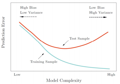
• Generalization of the classifier (model) The performance of the classifier on test data

Bayesian

• Bayes' Theorem: $$ P(A|B) = \frac{P(B\mid A)P(A)}{P(B)} $$

• Decision rule with only the prior information Decide $\omega_1$ if $P(\omega_1)\gt P(\omega_2)$, otherwise decide $\omega_2$

• Likelihood $P(x\mid \omega_j)$is called the likelihood of $\omega_j$ with respect to $x$; the category $\omega_j$ for which $P(x\mid \omega_j)$ is large is more likely to be the true category

• Maximum likelihood decision Assign input pattern $x$ to class $\omega_1$ if $P(x \mid \omega_1) > P(x \mid \omega_2),$ otherwise $\omega_2$

• Posterior $$ P(\omega_i\mid x)=\frac{P(x\mid \omega_i)P(\omega_i)}{P(x)}\ P(x)=\sum_{i=1}^{k}{P(x\mid \omega_i)P(\omega_i)} $$ Posterior = (Likelihood × Prior) / Evidence

• Optimal Bayes Decision Rule Decision given the posterior probabilities, Optimal Bayes Decision rule Assign input pattern $x$ to class $\omega_1$ if $P(\omega_1 \mid x) > P(\omega_2 \mid x),$ otherwise $\omega_2$ Bayes decision rule minimizes the probability of error, that is the term Optimal comes from. $$ P(error\mid x) = \min{\left{P(\omega_1\mid x),P(\omega_2\mid x)\right}} $$

• Special cases:

  1. if $P(\omega_1)=P(\omega_2)$, decide $\omega_1$ if $P(x\mid \omega_1)\gt P(x\mid \omega_2)$, otherwise $\omega_2$. (MLD)
  2. if $P(x\mid \omega_1) = P(x\mid \omega_2)$, decide $\omega_1$ if $P(\omega_1)\gt P(\omega_2)$, otherwise $\omega_2$.

• Bayes Risk

  • Conditional risk $\alpha_i$ is action and $\lambda(\alpha_i\mid \omega_i)$ is he loss incurred for taking action $\omega_i$ when the true state of nature is $\omega_j$. $$ R(\alpha_i \mid \boldsymbol{x}) = \sum_{j=1}^{c}{\lambda(\alpha_i\mid \omega_j)P(\omega_j\mid \boldsymbol{x})} $$
  • Bayes Risk $$ R=\sum_{\boldsymbol{x}}{R(\alpha_i\mid \boldsymbol{x})} $$
  • Minimum Bayes risk = best performance that can be achieved

• Likelihood Ratio if $$ \frac{P(\boldsymbol{x}\mid\omega_1)}{P(\boldsymbol{x}\mid\omega_2)}\gt \frac{\lambda_{12}-\lambda_{22}}{\lambda_{12}-\lambda_{11}} \times \frac{P(\omega_2)}{P(\omega_1)} $$ decide $\omega_1$. "If the likelihood ratio exceeds a threshold value that is independent of the input pattern x, we can take optimal actions"

• Minimum Error Rate Classification $$ R(\alpha_x\mid \boldsymbol{x}) = 1-P(\omega_i\mid \boldsymbol{x}) $$ Minimizing the risk → Maximizing the posterior $P(\omega_i\mid \boldsymbol{x})$

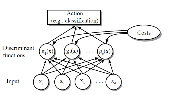
• Network Representation of a Classifier

• Bayes Classifier $$ g_i(\boldsymbol{x}) = P(\boldsymbol{x}\mid \omega_i)P(\omega_i)\ g_i(\boldsymbol{x}) = \ln{P(\boldsymbol{x}\mid \omega_i)}+\ln{P(\omega_i)} $$

• Binary classification → Multi‐class classification

  • One vs. One
  • One vs. Rest
  • ECOC

• Normal Distribution $\cal{N}(\boldsymbol{\mu}, \Sigma)$(with dimension $d$) $$ P(\boldsymbol{x})= \frac{1}{\left(2\pi\right)^{\frac{d}{2}}\left|\Sigma\right|^{\frac{1}{2}}}{\exp{\left[-\frac{1}{2}\left(\boldsymbol{x}-\boldsymbol{\mu}\right)^T\Sigma^{-1}\left(\boldsymbol{x}-\boldsymbol{\mu}\right)\right]}} $$

• Maximum‐Likelihood Estimation

  • Gradient operator $$ \nabla_{\theta}=\left[\frac{\partial}{\partial\theta_1},\cdots,\frac{\theta}{\partial\theta_p}\right] $$
  • Optimal Estimation $$ \nabla_\theta l=\sum_{k=1}^{n}\ln{P(x_k\mid\theta)}=0 $$

• Gaussian with unknown $\mu$ and $\Sigma$ $$ \boldsymbol{\hat{\mu}}=\frac{1}{n}\sum_{k=1}^{n}\boldsymbol{x}k\ \boldsymbol{\hat{\Sigma}}=\frac{1}{n}\sum{k=1}^{n}{\left(\boldsymbol{x}_k-\boldsymbol{\hat{\mu}}\right)\left(\boldsymbol{x}_k-\boldsymbol{\hat{\mu}}\right)^T} $$

• Bayesian Estimation $$ P(\omega_i\mid \mathbf{x}, \mathcal{D})=\frac{p(\mathbf{x}\mid \omega_i, \mathcal{D}i)P(\omega_i)}{\sum{j=1}^c{p(\mathbf{x}\mid \omega_j, \mathcal{D}_j)P(\omega_j)}} $$ where $$ p(x\mid D)=\int{p(x,\theta\mid D)d\theta}=\int{p(x\mid\theta, D)p(\theta\mid D)d\theta}\ =\int{p(x\mid \theta)p(\theta\mid D)d\theta} $$ $P(x\mid D)$ is the central problem of Bayesian learning.

  • General Theory $P(x \mid D)$ computation can be applied to any situation in which the unknown density can be parameterized: the basic assumptions are:
    • The form of $P(x \mid\theta)$ is assumed known, but the value of $\theta$ is not known exactly
    • Our knowledge about $\theta$ is assumed to be contained in a known prior density $P(\theta)$
    • The rest of our knowledge about $\theta$ is contained in a set D of n random variables $x_1, x_2, \dots, x_n$ that follows $P(x)$

• Linear Discriminant Analysis Covariance matrices of all classes are identical but can be arbitrary $$ g_i(x)=\mu_i^T\Sigma^{-1}x-\frac{1}{2}\mu_i^T\Sigma^{-1}\mu_i+\ln{P(\omega_i)} $$

  • Estimating Parameters:
    • $\mu_i$ $$ \mu_i=\frac{1}{N_i}\sum_{j\in\omega_i}x_j $$
    • $P(\omega_i)$ $$ P(\omega_i)=\frac{N_i}{N} $$
    • $\Sigma$ $$ \Sigma=\sum_{i=1}^c\sum_{j\in\omega_i}\frac{\left(\boldsymbol{x}_j-\boldsymbol{\mu_i}\right)\left(\boldsymbol{x}_j-\boldsymbol{\mu_i}\right)^T}{N_i} $$

• Error Probabilities and Integrals $$ P(error)=\int_{R_2}{p(x\mid\omega_1)P(\omega_1)dx}+\int_{R_1}{p(x\mid\omega_2)P(\omega_2)dx} $$

• Naive Bayes Classifier $$ P(\omega\mid x_1,\dots,x_p)\propto P(x_1,\dots, x_p\mid \omega)P(\omega)\ P(x_1,\dots,x_p\mid \omega)=P(x_1\mid \omega)\cdots P(x_p\mid \omega) $$

• Smoothing $$ P(x_i\mid \omega_k)=\frac{\left|x_{ik}\right|+1}{N_{\omega k}+K} $$

Perception

• Perceptron $$ f(x)=w^Tx+w_0\ y=sign(f(x)) $$
  • Learn
    • If correct, do nothing
    • If wrong, $w_t=w_{t-1}+xy$
• Perceptron Criterion Function $$ E(w)=-\sum_{i\in I_M}w^Tx_iy_i $$
• Gradient Descent (Steepest descent) $$ x_{n+1}=x_n-\gamma\nabla f(x_n),n\geqslant0 $$ Let $J(w)$be the criterion function. $$ w(k+1)=w(k)-\eta(k)\nabla J(w(k)) $$
• Batch learning vs. Online learning
  • Batch learning All the training samples are available
  • Online learning The learning algorithm sees the training samples one by one.
• Perceptron Convergence
  • converge if the data is linearly separable.
  • infinite loop if the training data is not linearly separable

Linear Regression

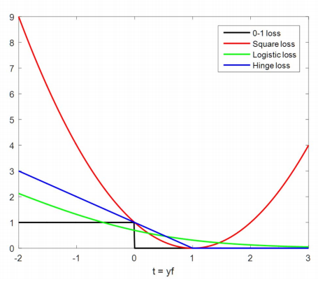
• Polynomial Curve Fitting $$ f(x, a)=\sum_{j=0}^M{a_jx^j}\ MSE(a)=\frac{1}{n}\sum_{i=1}^n{(y_i-f(x_i, a))^2}\ RSS(a)= \sum_{i=1}^n{(y_i-f(x_i, a))^2} $$
• Linear Regression Model $$ J_n(a)=(y-X^Ta)^T(y-X^Ta) $$
  • Gradient Descent $$ a_{k+1}=a_k+\eta_k2X(X^Ta-y) $$
  • fitted values $$ \hat{y}=X^Ta=X^T(XX^T)^{-1}Xy $$
• Statistical model of regression
  • A generative model: $y=f(x,a)+\epsilon$, where $\epsilon\sim N(0,\sigma^2)$. The maximum likelihood estimation result is approximate to RSS.
• Overfitting if $XX^T$$ is singular, overfitting.
• Ridge Regression $$ a^\star = argmin{\sum_{i=1}^n{(y_i-f(x_i, a))^2}+\lambda\sum^p_{j=1}a_j^2}\ a^\star=(XX^T+\lambda I)^{-1}Xy $$
• Maximum Likelihood Estimation If the prior is chosen as: $$ p(a)=\mathcal{N}(a\mid 0, \lambda^{-1}I) $$ then it's also a ridge regression.
• Bias‐variance Decomposition Expected prediction error (expected loss) = (bias)²+variance+noise
• The Bias‐Variance Trade‐off
  • Over‐regularized model (large λ) → high bias
  • Under‐regularized model (small λ)→ high variance
• LASSO
  • Using one norm as regularization
  • Sparse model

Logistic Regression

• Sigmoid function $$ \sigma(t)=\frac{1}{1+e^{-t}} $$
• Logistic Regression $$ P(y_i=\pm1\mid x_i, a)=\frac{1}{1+e^{-y_ia^Tx_i}} $$
• Criterion function $$ E(a)=\sum_{i\in I}{\log(1+e^{-y_ia^Tx_i})} $$

SVM

• Geometrical Margin $$ \gamma = y\frac{w^Tx+b}{\left|w\right|} $$
• Maximum Margin Classifier
  • Maximize the confidence of classifying the dataset
  • Criterion function let $w^Tx+b=1$. $$ \min_{w,b}{\left|w\right|}\ \Rightarrow \min_{w,b}{\frac{1}{2}\left|w\right|^2}\ s.t. y_i(w^Tx+b)\geqslant 1 $$
  • Support Vectors $$ y_i(w^Tx+b) = 1 $$
• Weakness of the Original Model
  • When an outlier appear, the optimal hyperplane may be pushed far away from its original/correct place.
  • Assign a slack variable $\xi$ to each data point. That means we allow the point to deviate from the correct margin by a distance of $\xi$
  • New Objective Function $$ \min_{w,b}{\frac{1}{2}\left|w\right|^2 + C\sum_{i=1}^n{\xi_i}}\ s.t. y_i(w^Tx+b)\geqslant 1-\xi_i\ \xi_i\geqslant0 $$
  • Hinge loss $$ \max{\left[1-y(w^Tx_i+b),0\right]}+\frac{1}{2C}\left|w\right|^2 $$
• A General formulation of classifiers
  • optimize function $$ \min_f\left{\sum_{i=1}^n{\mathcal{l}(f)+\lambda R(f)}\right} $$
  • loss

Kernel

• Quadratic Discriminant Function $$ g(x)=w_0+\sum_{i=1}^d{w_ix_i}+\sum_{i=1}^d\sum_{j=1}^d{w_{ij}x_ix_j} $$ $g(x)=0$ represents a hyperquadric.
• Generalized Discriminant Function $$ g(x)=\sum_{i=1}^{\hat{d}}{a_iy_i(x)} $$ and $\mathbf{y}=[y_i]$ is called augmented feature vector. The element function is called the phi‐function.
• Representer Theorem ... admits a representation of form: $$ f(x)=\sum_{i=1}^m{\alpha_ik(x_i,x)} $$
• Kernelized Ridge Regression $$ \alpha = (X^TX+\lambda I)^{-1}y\ \hat{f}(x)=\sum_{i=1}^n{\alpha_ik(x_i,x)}\ k(x_i, x)=w^Tx=x^T_ix $$
• Kernels Let $k(x,x') \geqslant0$ be some measure of similarity between objects $x,x'\in \mathcal{X}$ where $\mathcal{X}$ is some abstract space; we will call $k$ a kernel function.
  • Typically the function is symmetric, and non‐negative
  • Linear kernels: $k(x,x')=x^Tx'$
  • Polynomial kernels: $k(x,x')=)x^Tx'+1)^d$
  • RBF kernels: $k(x,x')=\exp{\left(-\frac{\left|x-x'\right|}{2\sigma^2}\right)}$

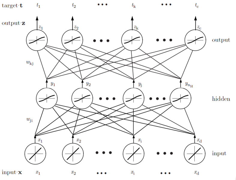
Neural Networks

• In using the multilayer neural Networks, the form of the nonlinearity is learned from the training data
• Multilayer neural network implements linear discriminants, but in a space where the inputs have been mapped nonlinearly
• Any continuous function from input to output can be implemented in a three‐layer net, given sufficient number of hidden units nH, proper nonlinearities, and weights
• Backpropagation Algorithm $$ \frac{\partial J}{\partial net_k}\cdot \frac{\partial net_k}{\partial w_{kj}}=-\delta_k\frac{\partial net_k}{\partial w_{kj}}\ \Delta w_{kj}=\eta\delta_ky_j $$
  • Stochastic: patterns are chosen randomly from training set; network weights are updated for each pattern
  • For each hidden unit, the weights from input layer describe the input pattern that leads to the maximum activation of that node

kNN & Decision Tree

• kNN Classifier
  • Use class labels of nearest neighbors to determine the class label of unknown record (e.g., by taking majority vote)
  • Effective number of parameters:$\frac{N}{K}$
• Decision Tree
  • A hierarchical data structure that represents data by implementing a divide and conquer strategy
  • Finding the minimal decision tree consistent with the data is NP‐hard
• Entropy $$ Entropy(S)=-\sum_{i=1}^c{P_i\log{P_i}} $$
  • If all the examples belong to the same category, Entropy=0
  • If the examples are equally mixed (0.5,0.5), Entropy=1
• Information Gain
  • The information gain of an attribute a is the expected reduction in entropy caused by partitioning on this attribute. $$ Gain(S,a)=Entropy(S)-\sum_{v\in values(a)}{\frac{\left|S_v\right|}{\left|S\right|}Entropy(S_v)} $$ where $S_v$ is the subset of $S$ for which attribute $a$ has value $v$.
• ID3 Choose the best attribute (highest gain)

Ensemble & Random Forest

• The Bagging Algorithm

  • Bootstrap sampling: re‐sample ܰN examples from D uniformly with replacement
  • Aggregating: adopts the most popular strategies for aggregating the outputs of the base learners, that is, voting for classification and averaging for regression.
  • bagging works reasonably well if base algorithm sensitive to data randomness
  • Variance is smaller: $$ \rho\sigma^2=\frac{1-\rho}{T}\sigma^2 $$ where T is smaples number, $\rho$ is correlation.
  • The base learner should aware the little change, sometimes overfitting is allowable

• Random Forest

  • uses decision tree as basic unit in bagging, is an ensemble model.
  • The main difference between the method of RF and Bagging is that RF incorporate randomized feature selection at each split step. $\sqrt{k}$ in classification and $k/3$ in regression.

• Boosting

  • Training base learners by assigning different weights to the samples. $$ \min_f\left{\sum_{i=1}^n{w_i\mathcal{l}(f)+\lambda R(f)}\right} $$

• AdaBoost

  1. $w_n^{(1)}=1/N$, for $n=1,\dots,N$.
  2. For $m=1,\dots,M$:
     1. Fit a classifier $y^{(m)}(x)$ to the training data by minimizing the weighted error function. $$ J_m=\sum_{n=1}^N{w_n^{(m)}I(y^{(m)}(x_n)\neq t_n)} $$
     2. Evaluate the Errorrate: $$ \epsilon_m=\frac{\sum_{n=1}^N{w_n^{(m)}I(y^{(m)}(x_n)\neq t_n)}}{\sum_{n=1}^N{w_n^{(m)}}} $$ and then use this to evaluate $$ \alpha_m=\ln{\frac{1-\epsilon_m}{\epsilon_m}} $$
     3. the data weighting coefficients $$ w_n={(m+1)}=w_n^{(m)}\exp{\left{\alpha_mI(y^{(m)}(x_n)\neq t_n)\right}} $$
  3. Make predictions using the final model, which is given by $$ Y_M(x)=sign\left(\sum_{m=1}^M{\alpha_my^{(m)}(x)}\right) $$

  weighting coefficients give greater weight to the more accurate classifiers when computing the overall output In each round, the algorithm try to get a different base learner, so that model diversity is achieved. $$ \frac{\sum_{n=1}^N{w_n^{(m+1)}I(y^{(m+1)}(x_n)\neq t_n)}}{\sum_{n=1}^N{w_n^{(m)}}}=\frac{1}{2} $$

• Optimization of Exponential Loss $$ E=\sum^N_{n=1}\exp{\left{-t_nf_m(x_n)\right}}, f_m(x)=\frac{1}{2}\sum_{i=1}^m{\alpha_ly_l(x)},t_n\in[-1,1] $$

Clustering

• K-means Given k, the k‐means algorithm is implemented in four steps:

  1. Partition objects into k nonempty subsets
  2. Compute seed points as the centroids of the clusters of the current partitioning
  3. Assign each object to the cluster with the nearest seed point
  4. Go back to Step 2, stop when he assignment does not change

• K-Medoids Instead of taking the mean value of the object in a cluster as a reference point, medoids can be used, which is the most centrally located object in a cluster.

• Partitioning Around Medoids (PAM) Calculate the pair‐wise distance matrix W first.

• Gaussian Mixture Model $$ p(x;\Theta)=\sum_{k=1}^K{\pi_kp_k(x;\theta_k)}\ \Theta=\left{\pi_1, \dots, \pi_k, \theta_1, \dots, theta_k\right}, \sum{\pi_k}=1\ p_k(x;\theta_k)=\mathcal{N}(x;\mu_k;\Sigma_k) $$ For each point $x^{(i)}$, $z^{(i)}$ associate with a hidden variable denotes $x^{(i)}$ which Gaussian $x^{(i)}$ belongs to

• EM algorithm $$ L(\theta)=\sum_{i=1}^m{\log{\sum_{z_{(i)}}{p(x^{(i)},z^{(i)};\theta)}}}\ =\sum_{i=1}^m{\log{\sum_{z_{(i)}}{Q^i(z^{i})\frac{p(x^{(i)},z^{(i)};\theta)}{Q^i(z^{i})}}}}\ \geqslant\sum_{i=1}^m{Q^i(z^{i})\sum_{z_{(i)}}{\log{\frac{p(x^{(i)},z^{(i)};\theta)}{Q^i(z^{i})}}}}=l(\theta) $$ Note that $f(x)=\log(x)$is a concave function and by Jensenʹs inequality, we have: $$ f\left(E_{z^{(i)}\sim Q}\left[\frac{p(x^{(i)},z^{(i)};\theta)}{Q^i(z^{i})}\right]\right)\geqslant E_{z^{(i)}\sim Q}\left[f\left(\frac{p(x^{(i)},z^{(i)};\theta)}{Q^i(z^{i})}\right)\right] $$ where the $z^{(i)}\sim Q$ subscripts above indicate that the expectations are with respect to $z^{(i)}$ drawn from $Q$. we'll make the inequality above hold with equality at our particular value of $\theta$.(E-step) $$ Q^i(z^{(i)})=p(z^{(i)}\mid x^{(i)};\theta) $$ So the fraction is constant that does not depend on $z^{(i)}$ $$ L(\theta_{n+1})\geqslant l_n(\theta_{n+1})\geqslant l_n(\theta_{n}=L(\theta_n) $$ Where $l_n(\theta_{n+1})$ means the lower‐bound function is computed with $Q_n$ parameterized by $\theta_{n+1}$. $l_n(\theta_{n+1})\geqslant l_n(\theta_{n})$ because $\theta_{n+1}=\arg\max_{\theta}l_n(\theta)$. In GMM, with $P(z^{(i)}=k)=\frac{\sum_k{Q_k^{(i)}}}{n}=\pi_k$. Q can be obtained by bayesian theorem.

• Spectral Clustering

  • Represent data points as the vertices V of a graph G.
    • All pairs of vertices are connected by an edge E.
    • Edges have weights W. Large weights mean that the adjacent vertices are very similar; small weights imply dissimilarity

  Divide vertices into two disjoint groups (A,B). Minimize weight of between‐group connections. $$ cut(A, B)= \sum_{i\in A, j\in B}{w_{ij}}\ assoc(A,V)=\sum_{i\in A, j\in V}{w_{ij}}\ \min Ncut(A, B)=\frac{cut(A,B)}{assoc(A,V)}+\frac{cut(A,B)}{assoc(B,V)} $$

• Objective Function of Ncut $$ D=[d_{ij}], d_{ii}=\sum_{j}{w_{ij}}\ \min_{y}{\frac{y^T(D-W)y}{y^TDy}}, y\in[2,-2b]^n, y^TD1=0 $$ where $$ k=\frac{\sum_{x_i>0}d_i}{\sum_id_i}, b=\frac{k}{1-k} $$

• Rayleigh quotient $$ \min_{y}{\frac{y^TLy}{y^TDy}}, y\in R^n, y^TD1=0\ \Rightarrow (D-W)y=\lambda Dy $$

• Generalized Eigen‐problem In this problem (with D and W), Vector 1 is the eigenvector corresponding to the eigenvalue 0. The eigenvector corresponding to the 2nd small eigenvalue. Each eigen vector (from small to large) of is a k dimensional representation of the original data point.

Dimensionality Reduction

$$ \mathcal{F}(x\in R^p)=z\in R^d $$ - if f is linear, linear dimensionality reduction $$ A^Tx=z $$ - Selection: choose a best **subset** of size d from the available p features - Extraction: given p features (set X), extract d new features (set Z) by linear or non‐linear combination of all the p features - PCA - Principal component analysis - Retains most of the sample's information. (large variance) - The new variables, called principal components, uncorrelated

$$
\max_{a}{a^TSa}, s.t. a^Ta=1 \\
\Rightarrow Sa=\lambda a
$$ where
$$
S=\frac{1}{n}{\sum_{i=1}^n{(x_i-\bar{x})(x_i-\bar{x})^T}}
$$ is the covariance matrix.
The kth largest eigenvalue of S is the variance of kth PC.

• Reconstruction $$ \bar{X}=A(A^TX) $$

• Optimality Property of PCA $$ \min_{A\in R^{p\times d}}{\left|X-AA^TX\right|^2_F}, s.t. A^TA=I_d $$ X is centered data matrix.

• LDA

  • Supervised
  • Linear Discriminant Analysis
  • Fisher Linear Discriminant
  • preserving asmuch of the class discriminatory information as possible

  $$ J(a)=\frac{(\tilde\mu_1-\tilde\mu_2)^2}{\tilde{s}^2_1+\tilde{s}^2_2}=\frac{a^TS_Ba}{a^TS_Wa} $$

  • within‐class scatter matrix: $S_W=S_1+S_2$.
  • between‐class scatter matrix: $S_B=(\mu_1-\mu_2)(\mu_1-\mu_2)^T$

  $$ S_Ba=\lambda S_Wa\ a^\star=S_W^{-1}(\mu_1-\mu_2) $$

  • Multi-class $$ J(a)=\frac{a^TS_Ba}{a^TS_Wa}\ S_W=\sum_{i=1}^cS_i\ S_B=\sum_{i=1}^c{n_i(\mu_i-\mu)(\mu_i-\mu)^T} $$

• LPP

  • Locality Preserving Projections

  • Graph W. L and D are the same as PCA.

  • Unsupervised, but it is very easy to have supervised (semi‐supervised) extensions. $$ \min{\sum_{ij}{w_{ij}(z_i-z_j)^2}}=\min{\frac{a^TXLX^Ta}{a^TXDX^Ta}}\ \Rightarrow XLX^Ta = \lambda XDX^Ta\ \Rightarrow XWX^Ta = \lambda XDX^Ta $$ when using L, smallest eigenvalue, when using W, largest eigenvalue.

  • LPP is equivalent to LDA when a specifically designed supervised graph is used

  • LPP is similar to PCA when an inner product graph is used. ($W=X^TX$)

  • Graph based Dimensionality Reduction $XWX^Ta = \lambda XDX^Ta$

  • Regularization: only max, add $\gamma I$ to the S in denominator(right side) (LDA, LPP).

• Laplacian Eigenmap $$ \min{y^TLy}\s.t. y^TDy=1 $$

TopicModel

• Document‐Term Matrix

• Query $$ cos(q,d)=\frac{q^Td}{\left|q\right|\left|d\right|} $$

• Polysemy: words with multiple meanings: sim < cos

• Synonymy: separate words that have the same meaning: sim > cos

• Language Model Paradigm $$ P(R_d=1\mid q)\propto P(q\mid R_d=1)P(R_d=1) $$

  • prior probability of relevance: uniform or popularity
  • query likelihood $$ P(q\mid d)=\prod_{w\in q}{P(w\mid d)} $$

• Naive Approach $$ \hat{P}(w\mid d)=\frac{n(d,w)}{\sum_{w'}{n(d, w')}} $$

• Probabilistic Latent Semantic Analysis $$ \hat{P}(w\mid d)=\sum_z{P(w\mid z)P(z\mid d)} $$

• Latent Dirichlet allocation ‐ adds a Dirichlet prior on the per‐document topic distribution, trying to address an often‐criticized shortcoming of PLSA, namely that it is not a proper generative model for new documents and at the same time avoid the overfitting problem.

Matrix Factorization

$$ UV=X $$ - Each column vector of ܺX can be represented as a linear combination of column vectors of U - Singular Value Decomposition (SVD) $$ X=U\Sigma V $$ where $$ U\in R^{m\times m}, V\in R^{n\times n}, UU^T=U^TU=I, VV^T=V^TV=1 $$ and $\Sigma$ is diagonal matrix. if rank(X)=d, $$ U\in R^{m\times d}, V\in R^{d\times n}, U^TU=I, VV^T=1 $$ and $\Sigma$ is diagonal matrix, usually **decrease**. - optimal low‐rank approximations $$ X^\star = \arg\min_{rank(\tilde{X})=k}{\left\|X-\tilde{X}\right\|} $$ - Relation to PCA Given an SVD of X, the following two relations hold: $$ X^TX=V(\Sigma^T\Sigma)V^T XX^T=U(\Sigma\Sigma^T)U^T $$ - Latent Semantic Analysis - Non‐negative Matrix Factorization useful in PLSA because, U and V requires positive. $$ X\cong \hat{X}=UV^T, u_{ij}\geqslant0, v_{ij}\geqslant 0 $$ - Euclidean distance $$ \left\|A-B\right\|^2=\sum_{ij}(A_{ij}-B_{ij})^2 $$ - Divergence $$ D(A\mid\mid B)=\sum_{ij}(A_{ij}\log{\frac{A_{ij}}{B_{ij}}}-A_{ij}+B_{ij}) $$ - Multiplicative Update Rules $$ u_{ik}\leftarrow \frac{(XV)_{ik}}{(UV^TV)_{ik}}u_{ik}\\ v_{jk}\leftarrow \frac{(XU)_{ik}}{(VU^TU)_{jk}}v_{jk} $$ - Sparse Coding $$ \min{\left\|X-UV^T\right\|^2_F+\lambda f(V)}, s.t. \sum_{i}u^2_{i,k}\leqslant c $$ Represent input vectors approximately as a weighted linear combination of a small number of “basis vectors.”